SYSTEMS OF LINEAR EQUATIONS

1. Systems of Linear Equations

Linear equations are by themselves not particularly interesting. More often than
not, one encounters collections of linear equations, involving the same variables,
which are to be considered simultaneously.

Definition. An m*n system of linear equations is a system of the form

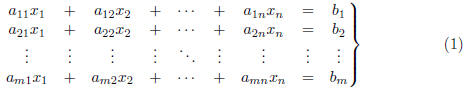
In particular, there are m equations in the n variables x₁, x₂, … , x_n. The numbers
a_ij are called the coefficients of the system (1) and the b_i are called the constant
terms.

Definition. A system of equations that has no solutions is called inconsistent. If
there is at least one solution of the given system, then it is called consistent.

In particular, note from the definition that a given linear system of equations
must be either consistent or inconsistent - there are no other possibilities.

Example 1. The 2*3 system

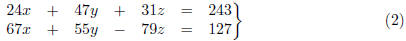
is consistent. This requires a brief geometric explanation (or a tedious calculation).

It turns out that the solution set of (2) corresponds to a line in R³. In particular,
we are asserting that there are infinitely many solutions to the system (2). Indeed,
the two equations determine two distinct planes in R³ which are not parallel (their
normal vectors (24, 47, 31) and (67, 55,-79) are not parallel since they are not
scalar multiples of each other). Geometrically, we know that two such planes in R³
must intersect each other and that this intersection must be a line.

See Figure 3.5.2 (p.157) of Anton which depicts the numerous ways in which three
planes in R³ might intersect. Have a close look at this drawing, since it illustrates
the geometry of all possible solution sets for 3*3 systems of linear equations.

Example 2. Consider the system

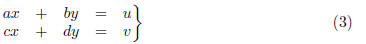
where a, b, c, d, u, v are constants and x, y are the variables. In terms of the familiar
slope-intercept formula for lines in the plane R², we can rewrite the system as

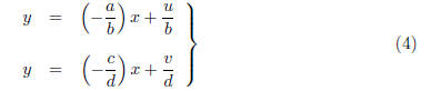
and regard these two equations as defining lines l₁ and l₂, respectively. It follows
that l₁ and l₂ are parallel (or possibly equal) when they have the same slope
(i.e., a/b = c/d). This is geometric condition is equivalent to the purely algebraic
condition

We can summarize this as follows:

(i) If ad - bc = 0, then there are two possibilities:

(a) l₁ and l₂ are parallel but not equal (i.e., they are distinct lines having
the same slope). In this case l₁ and l₂ do not intersect and hence the
system (3) has no solutions (the system is therefore inconsistent).

(b) l₁ and l₂ are in fact the same line and there are infinitely many
solutions to the system (3) exist (the system is therefore consistent).

(ii) If ad-bc ≠ 0, then l₁ and l₂ have different slopes and hence must intersect
and exactly one point, say (x₀, y₀). Thus the system (3) has exactly one
solution (the system is therefore consistent).

Of course, we need no geometry whatsoever to consider the system (3). Indeed,
you have all solved systems consisting of two equations in two unknowns before.
Nevertheless, thinking about things geometrically often helps our intuition and
helps us "picture things." For instance, now it is geometrically clear why the
mysterious quantity ad - bc arises in the consideration of 2*2 linear systems.

For 2*2 systems of the form (3), the quantity ad - bc is so important that it
has a special name:

Definition. The determinant of a 2*2 system of the form (3) is defined to be the
real number ad - bc.

We will discuss the determinants of n*n systems in the near future. However,
for the moment we would like to concentrate on some qualitative aspects of linear
systems. In particular, we remark that all of our examples have illustrated the
following (see Theorem 1.6.1 of Anton):

Theorem 1. A system of linear equations either has no solutions, exactly one
solution, or infinitely many solutions.

It is important to note that the preceding theorem only applies to linear systems
of equations. Indeed, nonlinear systems can have any number of solutions. For
instance, the nonlinear equation x² = 1 (i.e., a system consisting of one nonlinear
equation in one variable) has two solutions. Systems of linear equations are quite
special { be careful never to assume that something that works for linear equations
will work for nonlinear equations.

Example 3. If a linear system has two distinct solutions, then it must have
infinitely many solutions. For instance, suppose that we have a system of 2345 linear
equations in 874 unknowns. If we can find just two distinct solutions to this system,
then we can (via the theorem) conclude that the system actually has infinitely
many solutions.

The book has numerous examples (see Section 1.2 of the text) showing how to
find the solution sets for various systems of linear equations. For this class you will
rarely be required to solve systems of equations larger than 3*3. On the other
hand, it is important to see and do enough examples to gain a level of familiarity
with linear systems.

2. Homogeneous Linear Systems

Definition. A system of linear equations is said to be homogeneous if the constant
terms are all zero. In other words, an m*n (i.e., m equations in n unknowns)
homogeneous system is one of the form

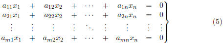
Observe that every homogeneous system is consistent since the trivial solution

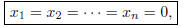
is obviously a solution to (5). Other solutions to the system (5), if they exist at all,
are referred to as nontrivial solutions.

Since a homogeneous linear system always has at least the trivial solution, it
follows (from Theorem 1) that exactly one of the following is true for a system of
the form (5):

(i) The system (5) has only the trivial solution
(ii) The system (5) has infinitely many solutions in addition to the trivial solution. In other words, the system has
infinitely many nontrivial solutions.

Example 4. Consider the general 2*2 homogeneous linear system below

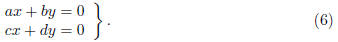
The two equations in (6) represent lines l₁ and l₂ in R² which pass through the origin
(0, 0). This corresponds to the fact that a homogeneous system of equations always
has at least the trivial solution. In fact, the only way that nontrivial solutions to
(6) can exist is if l₁ = l₂. This is because l₁ and l₂ are guaranteed to meet at the
origin - if they intersect elsewhere, then they must actually be the same line.

Recall that if ad - bc = 0, then l₁ and l₂ have the same slope. Since l₁ and l₂
have the same y-intercept (namely y = 0) it follows that ad - bc = 0 means that
l₁ = l₂. In other words:

(i) If ad-bc = 0, then (6) has infinitely many nontrivial solutions (in addition
to the trivial solution x = y = 0).

(ii) If ad-bc ≠ 0, then (6) has exactly one solution, namely the trivial solution.

The fact that (6) is homogeneous is crucial here. If the constant terms were
not both zero, then l₁ and l₂ could have the same slope (i.e., ad - bc = 0) yet not
intersect at all (they could be parallel to each other).

Another important fact about homogeneous linear systems is the following:

Theorem 2. A homogeneous system of linear equations with more unknowns than
equations must have infinitely many solutions.

It is important to note that the preceding theorem (Theorem 1.2.1 of the text)
applies only to homogeneous systems (see problem 1.2.28 of Anton).

Example 5. A system of the form

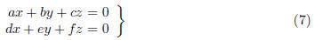
(where a, b, c, d, e, f are constants and x, y, z are the variables) always has infinitely
many solutions. Indeed, geometrically, the preceding equations represent two planes
P₁ and P₂ in R³. Since the system is homogeneous, both P₁ and P₂ pass through
the origin (0, 0, 0) - in other words P₁ and P₂ are guaranteed to intersect (contrast
this with the inhomogeneous case). This is because the trivial solution

x = y = z = 0

is automatically a solution to both equations in the system (7). Geometrically, we
can see that either P₁ = P₂ or P₁ and P₂ intersect in a straight line. In either case,
there are infinitely many solutions to the system (7).