Solving a Quadratic Equation

The most important points and skills for Section 2.5:

• Given the graph, table, or formula of a function, students should be able to determine the concavity of
the graph over a given interval by calculating average rates of change over specified intervals and noting
that the average rates of change increase (concave up) or decrease (concave down).

• Given the graph of a function that is either always concave up or always concave down, students should
be able to use secant lines between regularly spaced x-values to explain why increasing rate of change
leads to a concave up graph and why a decreasing rate of change leads to a concave down graph.

• Students must be aware that increasing/decreasing and concave up/down are fundamentally different
properties of a function – for example, just because a function is increasing does not mean that it is
concave up.

The most important points to take out of Section 2.6:

• Students should know that the formula for a quadratic equation resembles y = ax^2 + bx + c, where a is
not equal to zero.

• Given the equation of a quadratic function, students should be able to predict whether the graph concave
up or down based on the sign (+ or −) of the leading coefficient, a.

• If students have a quadratic equation and are given an x-value, then they should be able to evaluate the
quadratic equation at the x-value, respecting the order of operations.

• Students should know that “solving” a quadratic equation of the form ax^2 + bx + c = 0 means to find the
“zeros” of the function; that is, all of the values of x that can be plugged into the left hand side of the
equation to produce an output value of zero. They should also realize the zeros are the x-values at which
the graph of y = ax^2 + bx + c crosses the x-axis.

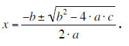
• Given a quadratic equation of the form: ax^2 + bx + c = 0, students should be able to find all solutions by
factoring into the form of a(x-r)(x-s)=0, or by substituting the values of a, b and c into the quadratic
formula:

0-20 Use this time to return any graded work (quizzes or team homework) and go over homework questions.
Be mindful of the time today since we will be covering 2 sections in the text (which is also why it would
be best not to do a quiz today). Section 2.4 #35 on page 83 is a homework problem of emphasis. If you
have time, go over the correct interpretations of these statements, paying close attention to the correct
use of units. If you do not have time to cover this problem in class, it would be a good idea to put a
similar problem on a quiz.

20-30 Lines are functions with constant rates of change. In this section we describe functions with increasing
or decreasing rates of change to introduce the concept of concavity. You could begin your introduction
to concavity with a simple example like the following: Consider the distances (in miles) traveled by two
cyclists, Mike and Eric, as a function of the time (t in hours). Begin by only filling in the first two
columns, and then have them fill in the third column.

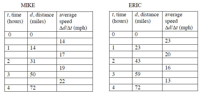
Ask the students to also graph the distances of each cyclist as a function of time. Ask them to make a
connection between the speeds of the cyclist and the shapes of the graphs. In particular, look for
statements noting that Mike’s speed increases and his distance graph bends up (is concave up), while
Eric’s speed decreases and his graph bends down (is concave down).

Wrap up this problem with the following question: If the cyclists’ trends continue, whom do we expect
to have traveled farther at the end of 5 hours?

30-40 One of the hardest ideas for students to grasp when working with tables and rates of change is to
understand why a function like y = x^2 (x < 0) is concave up from the calculation of average rates of
change. The point that the students often miss is that although the rates of change are getting smaller in
magnitude, when you taken into account that the rates of change are negative, they actually turn out to
be increasing (and the function concave up). You could graphically represent this by drawing y=x^2 on
the board and drawing the secant lines between x = -2 and x = -1, between -1 and 0, 0 and 1, etc.

To demonstrate this concept with tables, you could ask the students to calculate the average rate between
successive intervals for the table in Section 2.5 Problem #2 on page 86 (as they just did in the cyclist
example) in order to figure out if the graph would be concave up, down, or neither.

40-45 Call on the students’ experience with the cyclist example and Section 2.5 #2 to emphasize that concave
up/down does not correlate with increasing/decreasing. You might sketch the four curves (Figures 2.22-
2.25) in the text on page 86.

45-55 Section 2.5 Problems #14 and #16 from page 87 provide good practice in translating verbal description
to a graph. Pick one of these problems, and have the students draw a graph in their groups. Then call on
groups to put the graph on the board and ask them to explain the shape. Make sure they label their axes
with an appropriate scale and units.

55-65 Next introduce quadratic functions, and their general form (y = ax^2 + bx + c). Point out that an important
characteristic of a quadratic function is that the average rate of change over equal intervals is not
constant (as in the case of linear functions), but is always changing. Students are generally familiar with
quadratic functions, so you may be able to move through some of this material quickly.

Define what it means to find the zeros of a function. Note that a quadratic function may have 0, 1, or 2
zeros. Take an example of a quadratic function that factors easily such as y = 3x^2 +5x – 2. Have the
students graph the function, and point out once again that the zeros of the function correspond to the x-intercepts
of the graph. Ask the students to factor the function into y = (3x-1)(x+2). Make sure they
understand how to algebraically solve for the zeros, and make sure their answers correlate with the zeros
on their graph.

Wrap up this problem by introducing the quadratic formula. Have the students confirm the answers they
just found by using it to find the zeros of y = 3x^2+5x-2.

Note: In Chapter 5, we will introduce the vertex form and the algorithm of “Completing the Square.”
You don’t need to tackle these topics today. After the book has introduced transformations of
functions in Chapter 5 we will take a closer look at why the vertex form of a quadratic function looks the
way it does – you don’t need to get into this today either.

65-80 The study of quadratic functions has many applications to physics. It is important to consider an
example of an object falling under the effect of gravity. Consider a ball that is thrown upward from a
bridge and is allowed to fall past the bridge all the way to the ground. For example let h(t) = -16t^2 +
42t + 120 denote the height of the ball in feet above the ground t seconds after being released. Make
sure that the students understand that the shape of the height graph does not represent the path of the
ball, which is straight up and down. Have them work in groups to answer the following questions:

1) How high is the ball when it is released?
2) When does the ball hit the ground? (Use the quadratic formula; are both answers valid?)
3) Sketch a graph of the function h. What is a meaningful domain and range for this problem? (Note that
the physical constraints of the situation restrict the domain and range to non-negative values.)
4) Solve h(t) = 100. Interpret the solution and illustrate it on your graph.

Before the class ends, remind the students that the Gateway deadline is approaching!